Anisotropic news

Numbers of directions, compared.

New paper out

Back in 2018 Aila, Claudia, Martina and I wrote a review piece listing the kind of statistics people use to describe directional structures in spatial point patterns (Rajala et al. 2018). Our plan was to gather what we could find into one toolbox, and then compare the tools with respect to statistical power, ease of use, and other such user-relevant metrics.

As we compiled and parsed the sparse literature, it became clear to us that due to the ambiguity of the null-hypothesis, a general test procedure for testing isotropy is probably always going to be a poorly defined construct. A point process can be isotropic only one way, but anisotropic in infinitely many ways. The process and the anisotropy mechanism might not be possible to separate, in general. A more specific problem is getting to the null-distribution of a chosen test statistics. Sampling from \(H_0\) under assumed isotropic generating model would be an option, but then we must ask how such a thing could be estimated under \(H_1\)? A geometric anisotropy mechanism would distort range parameter estimates, for example. An alternative is to side-step the model and emulate interesting parts of the process as if it where isotropic (Wong and Chiu 2016). But here again the distortion would muddle the waters. Perhaps it is best to go back to the field and collect more replicates (Redenbach et al. 2009).

Since we are academics and don’t like going to the fields, it is perfectly sensible for us to still compare the plethora of proposed statistics, i.e. the numbers we compute from the patterns, using simulations. We simply set the truth, say model \(\mathbf{x}_0\sim M_0\), from which we observe data patterns \(\{\mathbf{x}\}\) that have been pushed trough some anisotropy-inducing transformations \(T:\{\mathbf{x}_0\}\mapsto\{\mathbf{x}\}\). Since we know \(M_0\), we have access to every null-model related quantity we need. Particularly, for any summary statistics that claims to measure anisotropy, we can compute its statistical power. Repeat for many statistics, apply to many, many models and transformations, and four years later we arrive to what we used to call the “Battle Paper” (Rajala et al. 2022).

Results in brief(s)

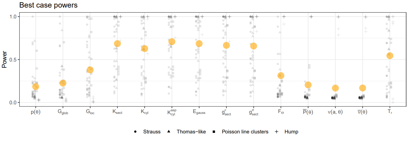
To roughly cover enough interesting types of patterns, in addition to the usual suspects of geometrically anisotropic Strauss and Thomas processes (heavily modified to have better control of point counts etc) we also included patterns with clear linear features, and a somewhat debatably relevant (non-stationary) patterns with single dense ridge running through the region. We included varying levels of point counts and strenghts of anisotropy, and computed most of the statistics described in the review paper. The end result was a very long list of powers that needed to be sifted for information.

The figure below gives the TL;DR, which is pretty much what one would expect when it comes to statistical power and point patterns: Pairwise stuff is more powerful than nearest neighbour stuff; Simple stuff is more powerful than complicated stuff. Various K-functions are pretty solid option almost always, and what flavour one chooses is more or less up to you, as long as you get the tuning parameters (opening angles, mostly) right. More details in the paper.

Overall results of the simulation trials. For each anisotropy summary, the gray points, with shape by model, give the best power over tuning parameters, integration limits, and tests. The large dot is the mean over all powers. (Figure 10 in the paper)

All the calculated statistics, and more what we discussed in the review paper but not in the battle paper, have been implemented (at varying degrees) in the R-package Kdirectional.

References

Rajala, T., C. Redenbach, A. Särkkä, and M. Sormani. 2018. “A Review on Anisotropy Analysis of Spatial Point Patterns.” Spatial Statistics 28 (December): 141–68. https://doi.org/10.1016/j.spasta.2018.04.005.

———. 2022. “Tests for Isotropy in Spatial Point Patterns A Comparison of Statistical Indices.” Spatial Statistics 52 (December): 100716. https://doi.org/10.1016/j.spasta.2022.100716.

Redenbach, Claudia, Aila Särkkä, Johannes Freitag, and Katja Schladitz. 2009. “Anisotropy Analysis of Pressed Point Processes.” AStA Advances in Statistical Analysis 93 (3): 237–61. https://doi.org/10.1007/s10182-009-0106-5.

Wong, Ka Yiu, and Sung Nok Chiu. 2016. “Isotropy Test for Spatial Point Processes Using Stochastic Reconstruction.” Spatial Statistics 15 (February): 56–69. https://doi.org/10.1016/j.spasta.2015.12.002.